Mechanistic Modeling of Bottom Water Dissolved Oxygen Dynamics in Baffin Bay
EPA Cooperative Agreement Numbers:
C6-48000053
EPA Q-TRAK#: 17-448
Coastal Bend Bays & Estuaries Program Contract No. 1729

Summary
Baffin Bay has been the subject of intensive water quality studies since 2013, largely in response to concerns over persistent algal blooms, fish kills, and hypoxic events. Over the past years, multiple water quality parameters, including dissolved oxygen (D.O.), nutrients (total dissolved inorganic nitrogen, phosphorous), chlorophyll-a (Chl-a), Secchi depth, organic carbon (both dissolved and particulate), and organic nitrogen (both particulate and dissolved) concentrations have been measured on a monthly basis by the Estuarine & Coastal Ecosystem Dynamics Lab at Texas A&M University - Corpus Christi with field assistance provided by the Baffin Bay Volunteer Water Quality Monitoring group. In addition, higher frequency (every 15 minutes, continuously) D.O. measurements commenced in early 2015.
Based on historical water quality monthly measurements, we developed a mechanistic dissolved oxygen model for Baffin Bay that tied together existing datasets (physical, chemical, and meteorological) obtained during the 2013-2016 period in an effort to examine the main drivers of D.O. dynamics and hypoxia formation in Baffin Bay. We found that water column D.O. was not sensitive to either respiration or photosynthesis within the water column, although bottom water was very sensitive to the sediment oxygen consumption because of the shallow water depth (~2 m). Scenario modeling that included various nutrient input conditions and temperature increases projected for the coming century was also conducted. Based on the model predictions, we found that warming has limited effect on water column D.O. changes. However, the ongoing eutrophication would enhance D.O. decrease, especially in the bottom waters. The outcome of this study is that it provides a science-based tool for management agencies and stakeholders for hypoxia mitigation purposes. This work revealed that curbing hypoxia highly depends on effective means to reduce nutrient loading into Baffin Bay.
Acknowledgemengts
We would like to thank the Texas Commission on Environmental Quality and the Coastal Bend Bays and Estuaries Program for supporting this project. Dr. Michael Wetz’s Estuarine & Coastal Ecosystem Dynamics Lab provided historical water quality data. Friends of Baffin Bay provided invaluable field assistance, which made the data collection available.Introduction
In recent years, hypoxia (dissolved oxygen or D.O. < 2mg L-1) was thought to be a possible cause for fish kills in Baffin Bay, a subtropical semiarid estuary in northwestern Gulf of Mexico (Wetz 2015). In general, coastal hypoxia is a result of increasing riverine anthropogenic nutrient input (Breitburg et al. 2018; Diaz and Rosenberg 2008; Kemp et al. 2009; Rabalais et al. 2009; Turner et al. 2006). Excessive nutrient loading to coastal waters enhances primary production and increases organic matter deposition in the sediment, thereby increasing oxygen consumption in both water column and surface sediment. Excessive organic matter production fuels aerobic respiration in the subsurface waters and sediment. At the same time, freshwater input can also increase vertical stratification due to water salt content difference (bottom water being saltier), which reduces the transfer of oxygen from surface to subsurface (Murphy et al. 2011; Rabalais et al. 2009; Zhang et al. 2017; Zhu et al. 2011). In addition, water column warming may also exacerbate hypoxic condition due to reduced oxygen solubility and stronger vertical stratification caused by temperature difference as surface water becomes warmer and less dense (Gruber 2011; Keeling et al. 2010). Because of the numerous physical and biogeochemical processes involved, a mechanistic model is a useful tool to understand the relative contributions of these different processes and elucidate which ones are dominant for hypoxia formation. Currently, there is no available model that describes oxygen dynamics in Baffin Bay. Therefore, it is imperative to develop such model for future management purposes including designing mitigation strategies and adaptation plans.
Baffin Bay has been the subject of intensive water quality studies since 2013, largely in response to concerns over persistent algal blooms, fish kills, and hypoxic events. As a part of these studies, various water quality parameters, including dissolved oxygen (D.O.), nutrients (total dissolved inorganic nitrogen and phosphorous), chlorophyll-a (Chl-a), Secchi depth, organic carbon (both dissolved and particulate), and organic nitrogen (both particulate and dissolved) concentrations have been measured on a monthly basis using the field assistance provided by the Baffin Bay Water Quality Monitoring group. In addition, higher frequency (every 15 minutes, continuously) D.O. measurements using Hydrolab multisondes commenced in early 2015 in both surface water (~50 cm below water surface) and bottom water (~30 cm above the bottom) at two locations in Baffin Bay (Fig. 1).
In this project, a mechanistic dissolved oxygen model was developed based on the water quality data, and this model tied together existing datasets (physical, chemical, and meteorological) produced during the 2013-2016 period in order to understand the main drivers of D.O. dynamics and hypoxia formation. The outcome of this work is that this modeling approach may provide a science-based tool for management agencies and stakeholders for hypoxia mitigation purposes and developing adaptation plans.
The D.O. model was based upon a previously published study for shallow stratified lakes and coastal waters (Stefan and Fang, 1994). We divided the water column in Baffin Bay into two layers when there was stratification. We assumed that each layer was horizontally well-mixed. The model was parameterized from the aforementioned monthly sample collections, and sediment D.O. consumption rates were measured through a previous Sea Grant-funded project entitled “Identification of Organic Matter Sources Contributing to Hypoxia Formation in Two Eutrophic South Texas Estuaries: Relationships to Watershed Land use Practices.” The produced model output was also used to compare with high-frequency continuous monitoring collected using in situ data sonde.
The model outputs generated contributions of different processes that are responsible for D.O. production and consumption. We used this information to unravel the dominant mechanisms involved in D.O. variability and hypoxia formation. Through scenario modeling (i.e., simulating increase in Chl-a levels, long-term water temperature changes), we proposed mitigation strategies for reducing the area of hypoxia in the Baffin Bay.
This project generated a high temporal resolution (daily) D.O. modeled dataset for different nutrient scenarios and temperature regimes. The data file contains the following columns of data:
- A date/time stamp (local standard time);
- Parameter value columns;
And the parameters reported include:
- Temperature
- Time stamp
- D.O.: dissolved oxygen concentration in mg L-1
Model Description
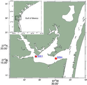
Fig. 1 A map of Baffin Bay and its relative location in the Gulf of Mexico. Water quality data used in the model construction were collected at two locations BB3 and BB6.
A two-dimensional D.O. budget model was developed to evaluate the mechanisms that control D.O. production and consumption in Baffin Bay. Two stations, BB3 (97?37.492'W 27?16.635'N) and BB6 (97?29.662'W 27?15.937'N) (Fig. 1) with monthly monitoring data, available since 2013, were used in this project.3�4 In this model, Baffin Bay water column with an average depth of ~2 m was divided into two layers (surface layer and bottom layer). We considered that each layer was horizontally well-mixed. The two-dimensionality assumption for both water temperature and D.O. is appropriate in Baffin Bay because horizontal water temperature and D.O. variation was much smaller than those in the vertical direction and across time (Stefan and Fang, 1994).
The change of D.O. in each layer was controlled by Eq. (1):
![]() (1)
(1)
here DO is the oxygen concentration in mg L-1 as a function of time (t). The parameters in Eq. (1) are explained in Table 1.
Table 1. Summary of fitting parameters in the DO budget model
| Symbol | Physical meaning | Required input parameters | Note |
| Fs | Air-sea flux across the air-water interface | Calculated from wind speed*, water temperature and salinity |
Zero for the bottom water non-zero for the surface water |
| Fb | Air sea flux due to bubbles | Calculated from wind speed*, water temperature and salinity |
Zero for the bottom water non-zero for the surface water |
| P | Oxygen source from photosynthesis | Calculated from PAR, Chl-a, nutrients, water temperature or lab measurement# |
|
| R | Oxygen sink from water column respiration |
Calculated from Chl-a, water temperature and salinity or lab measurement# |
|
| SOC | Sediment oxygen consumption | Lab measurement& | |
| Do | Vertical oxygen fluxes | Water temperature and salinity gradients | Zero when there is no stratification |
* Wind speed data are obtained from Naval Air Station Kingsville (automated airport weather observations with public access).
#
Monthly data are available from the ECEDL (TAMUCC).
& Monthly data are available from the Carbon Cycle Lab (TAMUCC).
Formulation of the D.O. Model
Surface reaeration due to air-sea exchange and bubbles (Fs+Fb)
Surface reaeration is one of the major sources for D. O. The diffusive exchange at the air-sea interface can be calculated by multiplying mass transfer coefficient, ks (m s-1), by the concentration difference between measured ([C], mol m-3) and equilibrium concentration that is determined by atmosphere gas partial pressure, [Cs]:
![]() (2)
(2)
Air-sea bubble flux (Fb) mainly includes two types of processes: the flux from small bubbles that totally collapse when they are forced below the air-sea interface (Fc), and that from larger bubbles that submerge, exchange gases and resurface, Fp.
![]() (3)
(3)
Fc and Fp were calculated based on a literature method (Emerson and Bushinsky 2016):
![]() (4)
(4)
![]() (5)
(5)
In Eqs. 4-5, kc and kp are mass transfer coefficients due to collapsing bubbles and exchange across large bubble interface, respectively; X is the atmospheric mole fraction of oxygen, DP is the fractional increase in pressure experienced by large bubbles and is a function of wind speed.
In this model, the total surface reaeration (FT) is the sum of the surface air-water flux, Fs, and the bubble flux, Fb:
![]() (6)
(6)
Oxygen production by photosynthesis (P)
Photosynthesis is an important oxygen production process and rate of photosynthesis depends on temperature, solar radiation, and nutrients availability (Eq. 7) (Stefan and Fang, 1994; Tian et al. 2014). In this model, we assumed that photosynthesis is a first-order kinetic process. Thus the oxygen production is proportional to the chlorophyll-a concentration (mg L-1), representing the biomass of phytoplankton.
![]() (7)
(7)
where Pmax is the maximum specific oxygen production rate by photosynthesis (mg O2 (mg Chl-a)-1 h-1), which is temperature dependent at saturating light conditions. Pmax is a function of temperature, which can be described using the Arrhenius equation (Eq. 8):
![]() (8)
(8)
In Eq. 7, Min[L] is the light limitation function and is a function of photosynthetically active radiation (PAR) and its attenuation in the water column as defined in Eq. 9:
![]() (9)
(9)
where α and β are the light-photosynthesis slope and light inhibition coefficient. µmax is the phytoplankton maximum growth rate. I represents the photosynthetically active radiation (PAR). Depth attenuation of I in the water column was calculated as a function of Chl-a concentration.
The limitation of phytoplankton growth by nitrogen and phosphate is formulated using the Michaelis
![]() (10)
(10)
where KN and KP are the half-saturation constants for nitrogen and phosphate uptake, respectively.
Respiration (R)
Aerobic respiration is the reverse reaction of photosynthesis, in which organic matter is transformed into inorganic matter by microbes under the existence of oxygen. We assumed respiration is a first-order kinetic process and related only to the concentration of Chl-a and temperature (Stefan and Fang, 1994):
![]() (11)
(11)
where kco is the ratio of Chl-a to oxygen utilized in respiration (both in the unit of mg L-1), Kr is the respiration rate coefficient (day-1), q is the temperature adjustment coefficient (Stefan and Fang, 1994).
Sediment oxygen consumption (SOC)
Sediment oxygen consumption rates have been measured with undisturbed surface sediment cores (~20 cm) and the data are available in the CCL for the 2015-2016 period.
Vertical diffusive flux (Do)
Tidal inflow and outflow were not considered in this model because of the very long water residence time in Baffin Bay (>1 yr) (Montagna et al. 2011), although the vertical mixing due to the tidal movement, surface wave and eddy turbulent diffusion contributes significantly to D.O. exchange between surface and bottom layer. The diffusive flux of oxygen (Do) is estimated from:
![]() (12)
(12)
In Eq. 12, Kz is the vertical eddy diffusivity and![]() is D.O. gradient along the pycnocline (Justić et al., 1996).
is D.O. gradient along the pycnocline (Justić et al., 1996).
Verification of D.O. model
The verification process for D.O. model consisted of two separate steps: model calibration and model validation. During the calibration step, the input coefficients for all the processes (Fs, Fb, P, R, SOC and D.O.) were adjusted to help the model to predict D.O. levels that matched the measured D.O. with an acceptable uncertainty (<1.0 mg L-1). The desired final calibration is a set of input coefficients that guarantee the model output meeting the acceptable uncertainty. If more than one set of coefficients meet all criteria, the optimal set of coefficients [Coeffcal] were selected based on the professional judgment of the modeler.It is noted that only a portion of total observed data were used in the calibration step. The remaining data were prepared for the validation process. For the validation step, the model prediction based on [Coeffcal] was quantitatively compared with the remaining validation data that spanned 2013-2016.
Results and Discussion
Model calibration
Given that temperature, salinity, nutrient, and Chl-a used to construct the model were only sampled monthly, daily values were re-calculated by linearly interpolating the nearest two sampling periods. Daily meteorological data were downloaded from the Kingsville Naval Air Station (http://mesonet.agron.iastate.edu/request/download.phtml?network=TX_ASOS).
We selected monthly data in 2015 (January-December) as the calibration dataset. The coefficients and parameters required by the calibration process were summarized in Table 2. Note that sediment D.O. consumption rate was linearly correlated with temperature (Fig. 2). Thus, its coefficients were directly derived from in situ measurements without further adjustment. During the calibration step, the input coefficients in Table 2 for all the processes (Fs, Fb, P, R, and D) were adjusted to help the model to predict D.O. levels, so that the model prediction could match the in situ measured D.O. within an acceptable uncertainty (�1.0 mg L-1).
Table 2. Values of the fitting parameters used in D.O. budget model
| Symbol | Physical meaning | Range |
Units |
|
| ks | Mass transfer coefficient for surface air-sea exchange |
(0.5~3)*10-5 | m s-1 | |
| kc | Mass transfer coefficient for exchange due to collapsing bubbles | (0.1~2)*10-8 | m s-1 | |
| kp | Mass transfer coefficient for exchange across large bubble interface | (0.1~6)*10-6 | m s-1 | |
| α | Light-photosynthesis slope | (0.5~3)*10-6 | m s-1 W-1 | |
| β | Light inhibition coefficient | (0.5~6)*10-8 | m s-1 W-1 | |
| �max | Phytoplankton maximum growth rate | (0.5~7)*10-5 | m s-1 | |
| KN | Half-saturation constant for nitrogen uptake |
0.1-1.0 | mmol N m-3 | |
| KP |
|
0.01-0.1 | mmol P m-3 | |
| Kco |
|
50-200 | - | |
| Kr |
|
0.05-0.6 | day-1 | |
| Kz |
|
(0.1~2.5)*10-4 | m2 s-1 | |
| θ | Temperature adjustment coefficient for respiration |
1.045-1.047 | - |
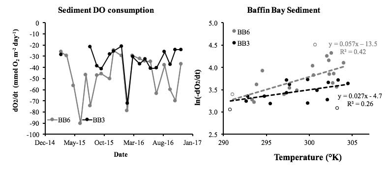
Fig. 2 Sediment D.O. consumption rate in Baffin Bay (a), and the relationship between sediment D.O. consumption and temperature (b). (Hover mouse to enlarage, click on the figure will lead to high resolution pdf version of the figure).
Generally, the model prediction matched well with the monthly average D.O. within the calibration dataset (Fig. 3). The regression coefficients R2 for Station BB6 was 0.73, which was higher than the value in Station BB3 (r2=0.61). However, the averaged residual of model prediction was -0.21 mg L-1 in Station BB6 and 0.09 mg L-1 in Station BB3. One of the reasons for both lower residual and R2 in Station BB3 was the limited seasonal cycle of D.O. concentration at Station BB3. Overall, the small model residual affirmed that the model predictions meet the allowable uncertainty criterion (�1.0 mg L-1) for calibration processes. Thus, we named the coefficients estimation from the calibration model as the “best-fit” reference value.
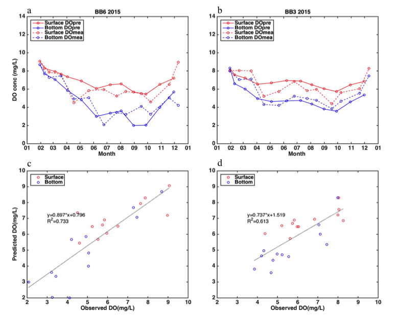
Fig. 3 Comparison between model prediction and monthly measurements based on the calibration dataset at both BB6 (a, c) and BB3(b, d).
Sensitivity analysis
Given air-sea exchange, photosynthesis, respiration, vertical diffusion, and sediment oxygen consumption all play a role on D.O. budget, the coefficients tested in the sensitivity analysis include wind speed, maximum specific oxygen production rate (Pmax), respiration rate coefficient (Kr), vertical diffusion rate (Kz), and sediment oxygen consumption rate (SOC). The sensitivity analysis was carried out by only changing one coefficient at a time from 75% to 125% of the best-fit reference value, while other coefficients were kept the same.
The results of the sensitivity tests indicate that surface D.O. was not sensitive to the changes in respiration rate coefficient Kr (Figs. 4a, 5a for BB6 and BB3, respectively) or photosynthetic production rate Pmax (Figs. 4c, 5c for BB6 and BB3, respectively) in both locations, because much of the surface oxygen replenishment came from air-sea exchange. However, bottom D.O. was very sensitive to vertical mixing (Figs. 4b, 5b) during warm months (July-October) and sediment oxygen consumption for the entire year (Figs. 4e, 5e). It is clear that sediment oxygen consumption was a very important D.O. sink for the bottom water, as indicated in the sensitivity analysis (Figs. 4e, 5e for BB6 and BB3, respectively). In addition, physical barriers that hindered vertical oxygen exchange, i.e., stratification, played a significant role in hypoxia formation in both locations (Figs. 4b, 5b for BB6 and BB3, respectively).
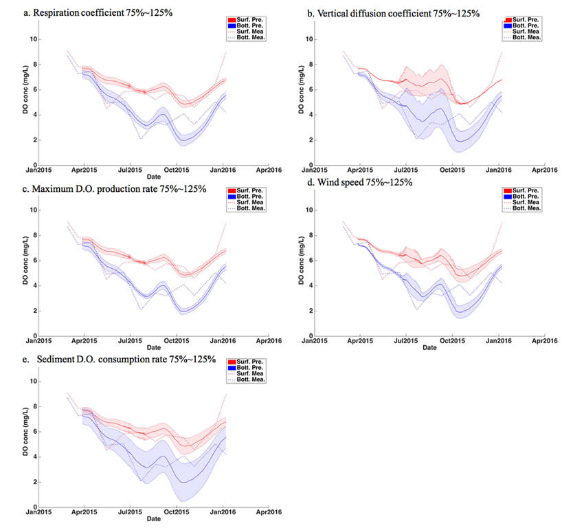
Fig. 4. Sensitivity analysis on the parameters and coefficients used in the D.O. model at Station BB6. The shaded areas represent the modeled standard deviation derived from changing the corresponding coefficients between 75~125% of the “best-fit” reference value. The dotted lines represent measured D.O. concentrations. Blue represents bottom water and red represents surface water.
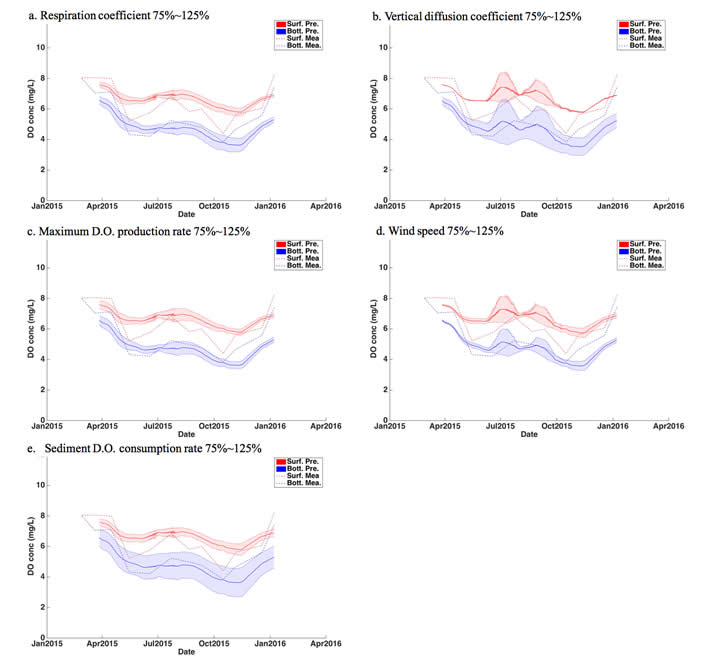
Fig. 5. Sensitivity analysis on the parameters and coefficients used in the D.O. model at Station BB3. The shaded areas represent the modeled standard deviation derived from changing the corresponding coefficients between 75~125% of the “best-fit” reference values. The dotted lines represent measured D.O. concentrations. Blue represents bottom water and red represents surface water.
Model Validation
In the sensitivity analysis based on the 2015 data only, we found that vertical mixing and sediment oxygen consumption were important for the D.O. prediction (Figs. 4, 5). Similar to the sensitivity tests above, we changed the key coefficients (wind speed, Pmax, Kr, Kz, and SOC) from 75% to 125% as the reference value and examined the entire 2013-2016 monthly data.
The multi-model predictions matched with the observed annual D.O. pattern very well with an average of 0.1�1.7 mg L-1 (mean � standard deviation). For example, the model predicted low bottom D.O. concentration in warm months, and nearly saturated D.O. concentration in cold months at Station BB6. In addition, the model also reproduced low surface water D.O. in summer months, which may have resulted from lower oxygen solubility at warm conditions and strong mixing between surface and bottom due to the shallow water depth. However, we suspect that the D.O. model has a limitation to predict D.O. under special physical conditions (i.e., well mixed condition), given the way that the vertical mixing was quantified. We assumed the vertical mixing was constant, which could be applied to most cases. However, when there was a strong, but short, period of mixing in Station BB6, the two-layer assumption did not hold any more, such as around summer 2014, when the model underestimated bottom D.O. at BB6 (Fig. 6a). Our D.O. model had a limitation in predicting the homogenous D.O. distribution at BB3 during the same period (Fig. 6b). Nevertheless, the low average residual (0.1�1.7 mg L-1) conffirmed that our model does not have bias and can predict the D.O. reasonably well. Note, given that monthly measured D.O. data were sufficient enough to do the calibration and validation, quarterly monitored D.O. data from TCEQ were thus not necessary for the model development.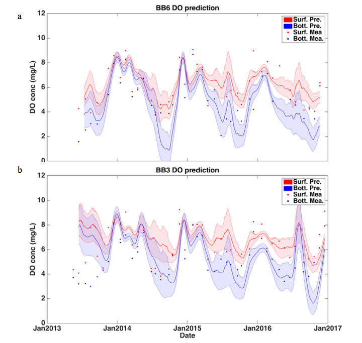
Fig. 6. Comparison between modeled and measurement D.O. concentration for the monthly monitoring dataset. The shaded area is the modeled standard deviation by changing the key coefficients by �25% of the “best-fit” values.
High frequency data
There was good agreement on salinity and temperature data collected from Baffin Bay Volunteer Water Quality Monitoring Study and high frequency sonde monitoring (Figs. 7a, b), despite the sporadic measurements of the latter. For example, the mean surface salinity and temperature differed 1.7 and -0.5 ?C in Station BB6 between these two datasets, respectively. Temperature has a clear seasonal cycle and ranged from ~10?C in December to ~31?C in August from 2015 to 2016.3�4 The seasonal variablity of salinity was remarkable because of the freshwater loading during April-May 2015. There was a salinity minimum from June to August 2015, which was recorded in both datasets. However, the higher frequency sonde dataset also recorded another salinity trough around June 2016, but the monthly sampling missed it. 3�4
In contrast to the good agreement between monthly sampling on salinity and temperature, the monthly collected D.O. did not match with the sonde data well (Fig. 7c), partitally resulting from the large daily varability. The sporadic high frequency D.O. data did not allow us to perform a thorough model validation. Nevertheless, the average differences between the D.O. model prediction and sonde data were 1.1�1.5 mg L-1 and -1.4�2.0 mg L-1 in surface and bottom layer, respectively. Comparing with the sonde data, the D.O. model overestimated D.O. in the surface water, but underestimated it in the bottom water. It is interesting that bottom D.O. concentration recorded by the sondes were occasionally higher than surface values, a phenomenon that was never recorded in the monthly dataset. One speculation is that this higher bottom D.O. could be caused by benthic microalgae (Blanchard and Montagna, 1992) or seagrass photosynthesis. However, given that the calibration data for the D.O. model did not have this benthic D.O. input term, it was thus difficult to incorporate this high-frequency dataset in the modeling for consideration.
Clearly, daily variation in D.O. recorded by the in situ sonde was greater than that from the model output, which was based on the linear interpolation of two adjacent monthly samplings. One important factor that contributed to this difference is that diel variability was not considered in the model. Instead the modeled data can be considered as daily average values. Nevertheless, the good agreement between the monthly monitoring data and the model prediction, based on a single year record, suggests that the developed model is suitable for examining D.O. dynamics.3�4 Although, the model’s predictive power may be enhanced when more high frequency data become available.
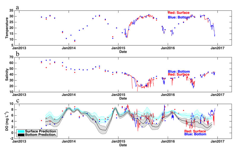
Fig. 7. Temperature, salinity and D.O. from both monthly and high frequency monitoring at Station BB6. Note, circles represent monthly measurements by the Baffin Bay Volunteer Water Quality Monitoring program; the red and blue lines are the daily average of surface and bottom within higher frequence sonde dataset; the cyan and black lines with the shaded area are D.O. model predictions in surface and bottom waters, respectively.
Future Scenarios
Using the D.O. model developed in this study, we predicted how D.O. in Baffin Bay would evolve under the ongoing warming and eutrophication conditions. We examined several scenarios by simulating the long-term water temperature changes (temperature +1?C), Chl-a concentration increased by 1.5 and 2 times from the present level. We elected to change one parameter at a time and kept other parameters the same. We assumed that the entire water column would warm up under the warming conditions, thus the thermocline itself would not change. Therefore, the warming would only change respiration, photosynthesis, and sediment oxygen consumption.
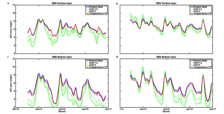
Fig. 8. The D.O. change under different scenarios at both Station BB3 and BB6.
Because D.O. was not sensitive to either respiration rate or maximum specific photosynthesis rate (Fig. 8), its concentration would only slightly decrease under the warming condition, mostly a result of decreased oxygen solubility. Although the sediment oxygen consumption was also related to temperature, the dependence was weak based on in situ incubations (Fig. 2). Therefore, warming itself would not decrease bottom D.O. significantly. In comparison, bottom D.O. is sensitive to the Chl-a change because the high Chl-a concentration corresponds to strong water and sediment oxygen consumption. This projection shows that both water column and bottom D.O. would continue to decrease with increasing eutrophication. At BB6 under the doubling of Chl-a scenario, even surface water could approach hypoxia (Fig. 8a) and bottom water would reach much more severe hypoxia (Fig. 8c&d). 3�4Thus, nutrient loading reduction should have the highest priority in managing the low D.O. conditions in Baffin Bay in the future warming climate.
Conclusions
In this project, we developed a mechanistic dissolved oxygen model for Baffin Bay using existing datasets (physical, chemical, and meteorological). Model construction utilized monthly monitoring water quality data from 2015 in the calibration step. Then the model validation step utilized remaining dataset from 2013-2016.
Overall, model prediction generated D.O. concentrations to be within 0.1�1.7 mg L-1 of the measured values. The modeling exercise suggested that water column D.O. was not sensitive to either respiration or photosynthesis. D.O. in the surface layer was dominated by air-sea exchange, vertical mixing, while the bottom water D.O. was sensitive to the sediment oxygen consumption.
Future warming only has limitation impact on the D.O. levels. However, eutrophication would play an important role in low D.O. formation in the water column. Therefore, curbing nutrient loading should remain a priority in mitigating hypoxia in Baffin Bay.
References
Blanchard, G.F. and Montagna, P.A., 1992. Photosynthetic response of natural assemblages of marine benthic microalgae to short- and long-term variations of incident irradiance in Baffin Bay, Texas. J. Phycol. 28(1),3�4 7-14.
Breitburg, D. et al. 2018. Declining oxygen in the global ocean and coastal waters. Science, 359(6371).
Diaz, R.J. and Rosenberg, R. 2008. Spreading dead zones and consequences for marine ecosystems. Science, 321(5891): 926-929.
Emerson, S. and Bushinsky, S. 2016. The role of bubbles during air-sea gas exchange. Journal of Geophysical Research: Oceans, 121(6): 4360-4376.
Gruber, N. 2011. Warming up, turning sour, losing breath: ocean biogeochemistry under global change. Philosophical Transactions of the Royal Society A: Mathematical, Physical and Engineering Sciences, 369(1943): 1980-1996.
Hopkinson, C.S. and Smith, E.M. 2005. Estuarine respiration: an overview of benthic, pelagic, and whole system respiration. In: P.A. del Giorgio and P.J.l.B. Williams (Editors), Respiration in Aquatic Ecosystems. Oxford University Press, pp. 122-146.
Justi?, D., Rabalais, N.N. and Turner, R.E., 1996. Effects of climate change on hypoxia in coastal waters: A doubled CO2 scenario for the northern Gulf of Mexico. Limnology and Oceanography, 41(5): 992-1003.
Keeling, R.F., Kortzinger2, A. and Gruber, N. 2010. Ocean deoxygenation in a warming world. Annual Review of Marine Science 2: 199-229.
Kemp, W.M., Testa, J.M., Conley, D.J., Gilbert, D. and Hagy, J.D. 2009. Temporal responses of coastal hypoxia to nutrient loading and physical controls. Biogeosciences, 6(12): 2985-3008.
Montagna, P., Vaughan, B. and Ward, G. 2011. The importance of freshwater inflows to Texas estuaries. In: R.C. Griffin (Editor), Water Policy in Texas: Responding to the Rise of Scarcity. The RFF Press, Washington D.C., pp. 107-127.
Murphy, R., Kemp, W. and Ball, W. 2011. Long-term trends in Chesapeake Bay seasonal hypoxia, stratification, and nutrient loading. Estuaries and Coasts, 34(6): 1293-1309.
Rabalais, N.N., Turner, R.E., D?az, R.J. and Justi?, D. 2009. Global change and eutrophication of coastal waters. ICES Journal of Marine Science: Journal du Conseil.
Stefan, H.G. and Fang, X., 1994. Dissolved oxgen model for regional lake analysis. Ecological Modelling, 71: 37-68.
Tian, R. et al. 2015. Model study of nutrient and phytoplankton dynamics in the Gulf of Maine: patterns and drivers for seasonal and interannual variability. ICES Journal of Marine Science, 72(2): 388-402.
Turner, R.E., Rabalais, N.N. and Justic, D. 2006. Predicting summer hypoxia in the northern Gulf of Mexico: Riverine N, P, and Si loading. Marine Pollution Bulletin, 52(2): 139-148.
Wetz, M.S. 2015. Baffin Bay Volunteer Water Quality Monitoring Study: Synthesis of May 2013-July 2015 Data. 1513, Texas A&M University-Corpus Christi.
Wetz, M.S. et al. 2017. Exceptionally high organic nitrogen concentrations in a semi-arid south Texas estuary susceptible to brown tide blooms. Estuarine, Coastal and Shelf Science, 188: 27-37.
Zhang, H., Zhao, L., Sun, Y., Wang, J. and Wei, H. 2017. Contribution of sediment oxygen demand to hypoxia development off the Changjiang Estuary. Estuarine, Coastal and Shelf Science, 192: 149-157.
Zhu, Z.-Y. et al. 2011. Hypoxia off the Changjiang (Yangtze River) Estuary: Oxygen depletion and organic matter decomposition. Marine Chemistry, 125(1
Appendices
3. Daily wind speed data from Kingsville Naval Air Station